Suraj Kurde

Sunday, 14 May 2017

Principles of Programming Languages - Blog

Savitribai Phule Pune University

Second Year Computer Engineering

2015 Pattern

Syllabus, Notes, PPT, Question Bank ..... click on link https://principalsofprogramminglanguagesse.wordpress.com/

Saturday, 28 January 2017

Write a function to get the number of vertices in an undirected graph and its edges. You may assume that no edge is input twice. i. Use adjacency list representation of the graph and find runtime of the function ii. Use adjacency matrix representation of the graph and find runtime of the function

/* C++ Program to Implement Graph using Adjacency List, Adjacency matrix, Traverse using BFS nd DFS */

#include <iostream>
#include <cstdlib>
#include<stdlib.h>
#include<list>
using namespace std;

int visited[20],visit[20],stk[20],top=0,qu[12],front,rear;

/* Adjacency List Node */
struct AdjListNode
{
    int dest;
    struct AdjListNode* next;
};

/* Adjacency List */
struct AdjList
{
    struct AdjListNode *head;
};

/* Class Graph */
class Graph
{
    private:
        int V,k;
        struct AdjList* array;
        int adjM[10][10];
        list<int>* adj;

    public:
        Graph(int V)
        {
            this->V = V;
            array = new AdjList [V];
            for (int i=1;i<=V; ++i)
            {
                      array[i].head = NULL;
                for(int j=1; j<=V; ++j)
                {
                adjM[i][j]=0;
                }
            }
            adj = new list<int>[V];
            for (int i=1; i<=V; ++i)
            visited[i]=0;
        }

        /* Creating New Adjacency List Node */

        AdjListNode* newAdjListNode(int dest)
        {
            AdjListNode* newNode = new AdjListNode;
            newNode->dest = dest;
            newNode->next = NULL;
            return newNode;
        }

        /*Add Edge to Graph */

   void addEdge()
        {
            int src,des;
            cout<<"\n Enter Edge ";
            cout<<"\n From -> ";
            cin>>src;
            cout<<"\n To -> ";
            cin>>des;
            adjM[src][des]=1;
            adjM[des][src]=1;
            adj[src].push_back(des);
            adj[des].push_back(src);
            AdjListNode* newNode = newAdjListNode(des);
            newNode->next = array[src].head;
            array[src].head = newNode;
            newNode = newAdjListNode(src);
            newNode->next = array[des].head;
            array[des].head = newNode;
        }

/* Print the graph*/

void printGraph()
        {
            int v;
        cout<<"\n Adjucency Matrix is : \n ";
        for (int i=1; i<=V; ++i)
        {
           for(int j=1; j<=V; ++j)
            {
               cout<<adjM[i][j]<<" ";
            }
        cout<<"\n";
        }
            for (v=1; v<=V;++v)
            {
                AdjListNode* p = array[v].head;
                cout<<"\n Adjacency list of vertex "<<v<<"\n head ";
                while(p)
                {
                   cout<<"-> "<<p->dest;
                    p = p->next;
                }
               cout<<endl;
            }
        }

/* Traverse using DFS   */
void DFS(int u)
    {
    for (int i=0;i<=V; ++i)
            visited[i]=0;
    int j;
    cout <<"ORDER OF VISITED VERTICES";
    cout << u <<" ";
    visited[u]=1;
    k=1;
    while(k<V)
    {
    for(j=V;j>=1;j--)
    {
    if(adjM[u][j]!=0 && visited[j]!=1 && visit[j]!=1)
    {
       visit[j]=1;
       stk[top]=j;
       top++;
    }
    }
    u=stk[--top];
    cout<<u << " ";
    k++;
    visit[u]=0; visited[u]=1;
    }
      }
/* Traverse using BFS   */
void bfs(int v)
{
for (int i=0;i<=V; ++i)
            visited[i]=0;
cout <<"Visitied vertices\n";
cout << v;
visited[v]=1;
k=1;
while(k<V)
{
for(int j=1;j<=V;j++)
if(adjM[v][j]!=0 && visited[j]!=1 && visit[j]!=1)
{
visit[j]=1;
qu[rear++]=j;
}
v=qu[front++];
cout<<v << " ";
k++;
visit[v]=0; visited[v]=1;
}
}

};

/* * Main */

int main()
{
    int ver,ed,ch,i,j,s;
    cout<<"Enter Count of No of Vertices";
    cin>>ver;

    cout<<"Enter Count of No of Egdes";
    cin>>ed;
    Graph gh(ed);
    do
    {
    cout<<"\n Select option :";
    cout<<"\n\t 1. Create graph \n \t2.Display graph \n\t3.DFS \n \t 4.BFS \n \t 5.Exit";
    cin>>ch;
    switch(ch)
    {
    case 1:
    for(i=0;i<ed;i++)
    gh.addEdge();
    break;
    case 2:
        // print the adjacency list representation of the above graph
            gh.printGraph();
        break;
    case 3:
            cout<<"\n select Initial Vertex";
            cin>>s;
        // print the adjacency list representation of the above graph
            gh.DFS(s);
        break;
    case 4:
            cout<<"\n select Initial Vertex";
            cin>>s;
        // print the adjacency list representation of the above graph
            gh.bfs(s);
        break;
    default : cout<<"\n Enter correct choice";
    }
    }while(ch!=5);

    return 0;
}

Saturday, 26 November 2016

About The Great Worrier "Shivaji Maharaj"

Shivaji Bhonsle (19 Feb 1630 – 3 April 1680), also known as Chhatrapati Shivaji Maharaj, was an Indian warrior king and a member of the Bhonsle Maratha clan. Shivaji carved out an enclave from the declining Adilshahi sultanate of Bijapur that formed the genesis of the Maratha Empire. In 1674, he was formally crowned as the Chhatrapati (Monarch) of his realm at Raigad.

Shivaji Maharaj established a competent and progressive civil rule with the help of a disciplined military and well-structured administrative organisations. He innovated military tactics, pioneering the guerrilla warfare methods (Shiva sutra or ganimi kava), which leveraged strategic factors like geography, speed, and surprise and focused pinpoint attacks to defeat his larger and more powerful enemies. He revived ancient Hindu political traditions and court conventions and promoted the usage of Marathi and Sanskrit, rather than Persian, in court and administration.

Shivaji Maharaj's legacy was to vary by observer and time but began to take on increased importance with the emergence of the Indian independence movement, as many elevated him as a proto-nationalist and hero of the Hindus. Particularly in Maharashtra, debates over his history and role have engendered great passion and sometimes even violence as disparate groups have sought to characterise him and his legacy.

Shivaji Maharaj was born in the hill-fort of Shivneri, near the city of Junnar in Pune district on 19 Feb. 1630. The Government of Maharashtra accepts 19 February 1630 as his birthdate; other suggested dates include 6 April 1627 or other dates near this day. Per legend, his mother named him Shivaji in honour of the goddess Shivai, to whom she had prayed for a healthy child. Shivaji was named after this local deity. Shivaji's father Shahaji Bhonsle was a Maratha general who served the Deccan Sultanates. His mother was Jijabai, the daughter of Lakhujirao Jadhav of Sindkhed (Sindkhed Raja). At the time of Shivaji's birth, the power in Deccan was shared by three Islamic sultanates: Bijapur, Ahmednagar, and Golconda. Shahaji often changed his loyalty between the Nizamshahi of Ahmadnagar, the Adilshah of Bijapur and the Mughals, but always kept his jagir (fiefdom) at Pune and his small army with him.

How to write Research Paper

Friday, 9 September 2016

Guassian membership Function in NN

%inputs
% XOR input for x1 and x2
input = [0 0; 0 1; 1 0; 1 1];
% Desired output of XOR
output = [0;1;1;0];
% Initialize the bias
bias = [-1 -1 -1];
% Learning coefficient
coeff = 0.7;
% Number of learning iterations
iterations = 10000;
% Calculate weights randomly using seed.
rand('state',sum(100*clock));
weights = -1 +2.*rand(3,3);

%with back propogation
for i = 1:iterations
   out = zeros(4,1);
   numIn = length (input(:,1));
   for j = 1:numIn
      % Hidden layer
      H1 = bias(1,1)*weights(1,1)
          + input(j,1)*weights(1,2)
          + input(j,2)*weights(1,3);

      % Send data through sigmoid function 1/1+e^-x
      % Note that sigma is a different m file
      % that I created to run this operation
      x2(1) = sigma(H1);
      H2 = bias(1,2)*weights(2,1)
           + input(j,1)*weights(2,2)
           + input(j,2)*weights(2,3);
      x2(2) = sigma(H2);

      % Output layer
      x3_1 = bias(1,3)*weights(3,1)
             + x2(1)*weights(3,2)
             + x2(2)*weights(3,3);
      out(j) = sigma(x3_1);

      % Adjust delta values of weights
      % For output layer:
      % delta(wi) = xi*delta,
      % delta = (1-actual output)*(desired output - actual output)
      delta3_1 = out(j)*(1-out(j))*(output(j)-out(j));

      % Propagate the delta backwards into hidden layers
      delta2_1 = x2(1)*(1-x2(1))*weights(3,2)*delta3_1;
      delta2_2 = x2(2)*(1-x2(2))*weights(3,3)*delta3_1;

      % Add weight changes to original weights
      % And use the new weights to repeat process.
      % delta weight = coeff*x*delta
      for k = 1:3
         if k == 1 % Bias cases
            weights(1,k) = weights(1,k) + coeff*bias(1,1)*delta2_1;
            weights(2,k) = weights(2,k) + coeff*bias(1,2)*delta2_2;
            weights(3,k) = weights(3,k) + coeff*bias(1,3)*delta3_1;
         else % When k=2 or 3 input cases to neurons
            weights(1,k) = weights(1,k) + coeff*input(j,1)*delta2_1;
            weights(2,k) = weights(2,k) + coeff*input(j,2)*delta2_2;
            weights(3,k) = weights(3,k) + coeff*x2(k-1)*delta3_1;
         end
      end
   end
end

Activation Function in NN

% Illustration of various activation functions used in NN's
x = -10:0.1:10;
tmp = exp(-x);
y1 = 1./(1+tmp);
y2 = (1-tmp)./(1+tmp);
y3 = x;
subplot(231); plot(x, y1); grid on;
axis([min(x) max(x) -2 2]);
title('Logistic Function');
xlabel('(a)');
axis('square');
subplot(232); plot(x, y2); grid on;
axis([min(x) max(x) -2 2]);
title('Hyperbolic Tangent Function');
xlabel('(b)');
axis('square');
subplot(233); plot(x, y3); grid on;
axis([min(x) max(x) min(x) max(x)]);
title('Identity Function');
xlabel('(c)');
axis('square');

Tuesday, 5 April 2016

Implement defuzzyfication (Max-membership principle, Centroid method, Weighted average method)

clc;
clear all;
close all;

ip=11;
a1=1;
a2=5;
b1=4;
b2=7;
c1=7;
c2=9;
d2=11;
s1=0;
s2=0;

%Triangular function

for u=1:ip
    if(u<=a1)
        t(u)=0;
    elseif((u>a1)&&(u<=b1))
        t(u)=((u-a1)/(b1-a1));
    elseif((u>b1)&&(u<=c1))
        t(u)=((c1-u)/(c1-b1));
    else
        t(u)=0;
    end
end

subplot(221)
plot(t);
title('Triangular Function');

%Pie function

for u=1:ip
    if(u<=a2)
        p(u)=0;
    elseif((u>a2)&&(u<=b2))
        p(u)=((u-a2)/(b2-a2));
    elseif((u>b2)&&(u<=c2))
        p(u)=1;
    elseif((u>c2)&&(u<=d2))
        p(u)=((d2-u)/(d2-c2));
    else
        p(u)=0;
    end
end

subplot(222)
plot(p);
title('Pie Function');

z=t+p;
subplot(223);
plot(z);

%Using Centroid Method
for i=1:11
    s1=s1+(z(i)*i);
    s2=s2+z(i);
end

op1=s1/s2;
disp('Using Centroid Method:');
disp(op1);

%Using Weighted average method
a=mean(ip);
s1=s1+t(a)*(a)+p(a)*(a);
s2=s2+z(a)+p(a);
op1=s1/s2;
disp('Using Weighted Average MEthod');
disp(op1);

%Using Max-Membership Principle
k=z(1);
m=1;
for i=2:ip
    if(k<z(i))
    k=z(i);
    m=i;
    end
end
disp('Using Max Membership principle');
disp(m);

Monday, 15 February 2016

Kohonen Self organizing feature map MATLAB code

clc;
clear all;
close all;

alpha=0.5;
x1=rand(1,100)-0.5;
x2=rand(1,100)-0.5;
x=[x1;x2];

w1=rand(1,50)-rand(1,50);
w2=rand(1,50)-rand(1,50);
w=[w1;w2];

figure(1);
plot([-0.5 0.5 0.5 -0.5 -0.5],[0.5 0.5 -0.5 -0.5 0.5]);
hold on;
plot(x1,x2,'b.');
axis([-1 1 -1 1]);

figure(2);
plot([-0.5 0.5 0.5 -0.5 -0.5],[0.5 0.5 -0.5 -0.5 0.5]);
hold on;
plot(w(1,:),w(2,:),'b.',w(1,:),w(2,:));
axis([-1 1 -1 1]);
hold off;
con=1;
ep=0;
while(con)
    for i=1:100
        for j=1:50
            d(j)=0;
            for k=1:2
                d(j)=d(j)+(w(k,j)-x(k,i))^2;
            end
        end
%         for j=1:50
%             if d(j)==min(d);
%                 J=j;
%             end
%         end
        [val J]=min(d);
        I=J-1;
        K=J+1;

        if(I<1)
            I=50;
        end

        if(K>50)
            K=1;
        end

        w(:,J)=w(:,J)+alpha*(x(:,i)-w(:,J));
        w(:,I)=w(:,I)+alpha*(x(:,i)-w(:,I));
        w(:,K)=w(:,K)+alpha*(x(:,i)-w(:,K));
    end

    alpha=alpha-0.0049;
    ep=ep+1;
    plot([-0.5 0.5 0.5 -0.5 -0.5],[0.5 0.5 -0.5 -0.5 0.5]);
    hold on;
    plot(w(1,:),w(2,:),'b*',w(1,:),w(2,:));
    axis([-1 1 -1 1]);
    pause(0.1);
    hold off;
    if(ep==100)
        con=0;
    end
end

figure(3);
plot([-0.5 0.5 0.5 -0.5 -0.5],[0.5 0.5 -0.5 -0.5 0.5]);
hold on;
plot(w(1,:),w(2,:),'b.',w(1,:),w(2,:));
axis([-1 1 -1 1]);

Tuesday, 2 February 2016

Implement perceptron for AND function using bipolar inputs

%Code

clc
clear all;
close all;

x1=[-1 -1 1 1];
x2=[-1 1 -1 1];
t=[-1 -1 -1 1];
alpha=input('Enter the value of alpha=');
th=input('enter the threshold=');
yin=zeros(1,4);
y=zeros(1,4);
w1=0;
w2=0;
b=0;
c=1;
cnt=0;
while(c)
    c=0
    for i=1:4
        %yin(i)=b+(x(i,1)*w1)+(x(i,2)*w2);
       yin(i)=b+(x1(i)*w1)+(x2(i)*w2);
        if yin(i)>th
            y(i)=1;
        else if yin(i)<-th
                y(i)=-1;
            else
                y(i)=0;
            end
            if t(i)~=y(i)
                w1=w1+(alpha*x1(i)*t(i));
                w2=w2+(alpha*x2(i)*t(i));
                b=b+(alpha*t(i));
                c=1;
            else
                w1=w1;
                w2=w2;
                b=b;
            end
        end
        cnt=cnt+1;
    end
    disp('OUTPUT MATRIX:');
    disp(y);
    disp('w1=');
    disp(w1);
    disp('w2=');
    disp(w2);
    disp('bias=');
    disp(b);
    a1=x1;
    a2=x2;
    a2=(-w1/w2)*a1-(b/w2);
    plot(x1,x2,'*r',a1,a2);
    axis([-2 2 -2 2]);
end

Wednesday, 13 January 2016

Implement fuzzy membership functions (triangular, trapezoidal, gbell, PI, Gamma, Gaussian) ......... MATLAB Code

clc;
clear all;
close all;

ip=input('Enter input range : ');
a=input('Enter value of alpha : ');
b=input('Enter value of beta : ');
c=input('Enter value of gamma : ');
d=input('Enter value of delta : ');
m=input('Enter value of m : ');
del=input('Enter value of del : ');

%Gamma function

for u=1:ip
    if(u<=a)
        g(u)=0;
    elseif((u>a)&&(u<=b))
        g(u)=((u-a)/(b-a));
    else
        g(u)=1;
    end
end

subplot(2,3,1)
plot(g)
title('Gamma Function')
axis([0 ip 0 1]);

%S function

for u=1:ip
    if(u<=a)
        s(u)=0;
    elseif((u>a)&&(u<=b))
        s(u)=2*(((u-a)/(c-a))^2);
    elseif((u>b)&&(u<=c))
        s(u)=1-(2*(((u-c)/(c-a))^2));
    else
        s(u)=1;
    end
end

subplot(2,3,2)
plot(s);
title('S Function');
axis([0 ip 0 1]);

%Triangular function

for u=1:ip
    if(u<=a)
        t(u)=0;
    elseif((u>a)&&(u<=b))
        t(u)=((u-a)/(b-a));
    elseif((u>b)&&(u<=c))
        t(u)=((c-u)/(c-b));
    else
        t(u)=0;
    end
end

subplot(2,3,3)
plot(t);
title('Triangular Function');
axis([0 ip 0 1]);

%Pie function

for u=1:ip
    if(u<=a)
        p(u)=0;
    elseif((u>a)&&(u<=b))
        p(u)=((u-a)/(b-a));
    elseif((u>b)&&(u<=c))
        p(u)=1;
    elseif((u>c)&&(u<=d))
        p(u)=((d-u)/(d-c));
    else
        p(u)=0;
    end
end

subplot(2,3,4)
plot(p);
title('Pie Function');
axis([0 ip 0 1]);

%Gaussian function

for u=1:ip
   gs(u)=exp((-((u-m)^2))/(2*(del^2)));
end

subplot(2,3,5)
plot(gs);
title('Gaussian Function');
axis([0 ip 0 1]);

Monday, 11 January 2016

Implement a simple linear regressor with a single neuron model .... MATLAB Code

// data.txt file

166, 54.00
195, 82.00
200, 72.00
260, 72.00
265, 90.00
335, 124.00
370, 94.00
450, 118.00

// .m file for linear regression

%Load the data from our text file
data = load('/home/svcet/Desktop/data.txt');
% Define x and y
x = data(:,2);
y = data(:,1);
% Create a function to plot the data
function plotData(x,y)
plot(x,y,'rx','MarkerSize',8); % Plot the data
end
% Plot the data
plotData(x,y);
xlabel('Cost of Book'); % Set the x-axis label
ylabel('Number of Pages'); % Set the y-axis label
fprintf('Program paused. Press enter to continue.\n');
pause;
% Count how many data points we have
m = length(x);
% Add a column of all ones (intercept term) to x
X = [ones(m, 1) x];
% Calculate theta
theta = (pinv(X'*X))*X'*y
% Plot the fitted equation we got from the regression
hold on; % this keeps our previous plot of the training data visible
plot(X(:,2), X*theta, '-')
legend('Training data', 'Linear regression')
hold off % Don't put any more plots on this figure

MLP trained with Backpropagation for XOR Function.... MATLAB Code

function y=binsig(x)
y=1/(1+exp(-x));
end

function y=binsig1(x)
y=binsig(x)*(1-binsig(x));
end

%Back Propagation Network for XOR function with Binary Input and Output
clc;
clear;
%Initialize weights and bias
v=[0.197 0.3191 -0.1448 0.3394;0.3099 0.1904 -0.0347 -0.4861];
v1=zeros(2,4);
b1=[-0.3378 0.2771 0.2859 -0.3329];
b2=-0.1401;
w=[0.4919;-0.2913;-0.3979;0.3581];
w1=zeros(4,1);
x=[1 1 0 0;1 0 1 0];
t=[0 1 1 0];
alpha=0.02;
mf=0.9;
con=1;
epoch=0;
while con
    e=0;
    for I=1:4
        %Feed forward
        for j=1:4
            zin(j)=b1(j);
            for i=1:2
                zin(j)=zin(j)+x(i,I)*v(i,j);
            end
            z(j)=binsig(zin(j));
        end
        yin=b2+z*w;
        y(I)=binsig(yin);
        %Backpropagation of Error
        delk=(t(I)-y(I))*binsig1(yin);
        delw=alpha*delk*z'+mf*(w-w1);
        delb2=alpha*delk;
        delinj=delk*w;
        for j=1:4
            delj(j,1)=delinj(j,1)*binsig1(zin(j));
        end
        for j=1:4
            for i=1:2
                delv(i,j)=alpha*delj(j,1)*x(i,I)+mf*(v(i,j)-v1(i,j));
            end
        end
        delb1=alpha*delj;
        w1=w;
        v1=v;
        %Weight updation
        w=w+delw;
        b2=b2+delb2;
        v=v+delv;
        b1=b1+delb1';
        e=e+(t(I)-y(I))^2;
    end
    if e<0.005
        con=0;
    end
    epoch=epoch+1;
end
disp('BPN for XOR funtion with Binary input and Output');
disp('Total Epoch Performed');
disp(epoch);
disp('Error');
disp(e);
disp('Final Weight matrix and bias');
v
b1
w
b2

Tuesday, 29 December 2015

Back-propagation Algorithm Example in Neural Network

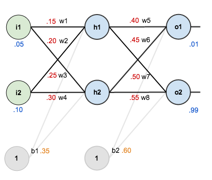
For this tutorial, we’re going to use a neural network with two inputs, two hidden neurons, two output neurons. Additionally, the hidden and output neurons will include a bias.
Here’s the basic structure:
neural_network (7)

In order to have some numbers to work with, here’s are the initial weights, the biases, and training inputs/outputs:
neural_network (9)

The goal of backpropagation is to optimize the weights so that the neural network can learn how to correctly map arbitrary inputs to outputs.
For the rest of this tutorial we’re going to work with a single training set: given inputs 0.05 and 0.10, we want the neural network to output 0.01 and 0.99.

The Forward Pass

To begin, lets see what the neural network currently predicts given the weights and biases above and inputs of 0.05 and 0.10. To do this we’ll feed those inputs forward though the network.
We figure out the total net input to each hidden layer neuron, squash the total net input using an activation function (here we use the logistic function), then repeat the process with the output layer neurons.

Total net input is also referred to as just net input by some sources.

Here’s how we calculate the total net input for $h_1$ :
$net_{h1} = w_1 * i_1 + w_2 * i_2 + b_1 * 1$
$net_{h1} = 0.15 * 0.05 + 0.2 * 0.1 + 0.35 * 1 = 0.3775$
We then squash it using the logistic function to get the output of $h_1$ :
$out_{h1} = \frac{1}{1+e^{-net_{h1}}} = \frac{1}{1+e^{-0.3775}} = 0.593269992$
Carrying out the same process for $h_2$ we get:
$out_{h2} = 0.596884378$
We repeat this process for the output layer neurons, using the output from the hidden layer neurons as inputs.
Here’s the output for $o_1$ :
$net_{o1} = w_5 * out_{h1} + w_6 * out_{h2} + b_2 * 1$
$net_{o1} = 0.4 * 0.593269992 + 0.45 * 0.596884378 + 0.6 * 1 = 1.105905967$
$out_{o1} = \frac{1}{1+e^{-net_{h1}}} = \frac{1}{1+e^{-1.105905967}} = 0.75136507$
And carrying out the same process for $o_2$ we get:
$out_{o2} = 0.772928465$

Calculating the Total Error

We can now calculate the error for each output neuron using the squared error function and sum them to get the total error:
$E_{total} = \sum \frac{1}{2}(target - output)^{2}$

Some sources refer to the target as the ideal and the output as the actual.

The $\frac{1}{2}$ is included so that exponent is cancelled when we differentiate later on. The result is eventually multiplied by a learning rate anyway so it doesn’t matter that we introduce a constant here [1].

For example, the target output for $o_1$ is 0.01 but the neural network output 0.75136507, therefore its error is:
$E_{o1} = \frac{1}{2}(target_{o1} - out_{o1})^{2} = \frac{1}{2}(0.01 - 0.75136507)^{2} = 0.274811083$
Repeating this process for $o_2$ (remembering that the target is 0.99) we get:
$E_{o2} = 0.023560026$
The total error for the neural network is the sum of these errors:
$E_{total} = E_{o1} + E_{o2} = 0.274811083 + 0.023560026 = 0.298371109$

The Backwards Pass

Our goal with backpropagation is to update each of the weights in the network so that they cause the actual output to be closer the target output, thereby minimizing the error for each output neuron and the network as a whole.

Output Layer

Consider $w_5$ . We want to know how much a change in $w_5$ affects the total error, aka $\frac{\partial E_{total}}{\partial w_{5}}$ .

$\frac{\partial E_{total}}{\partial w_{5}}$ is read as “the partial derivative of $E_{total}$ with respect to $w_{5}$ “. You can also say “the gradient with respect to $w_{5}$ “.

By applying the chain rule we know that:
$\frac{\partial E_{total}}{\partial w_{5}} = \frac{\partial E_{total}}{\partial out_{o1}} * \frac{\partial out_{o1}}{\partial net_{o1}} * \frac{\partial net_{o1}}{\partial w_{5}}$
Visually, here’s what we’re doing:
output_1_backprop (4)

We need to figure out each piece in this equation.
First, how much does the total error change with respect to the output?
$E_{total} = \frac{1}{2}(target_{o1} - out_{o1})^{2} + \frac{1}{2}(target_{o2} - out_{o2})^{2}$
$\frac{\partial E_{total}}{\partial out_{o1}} = 2 * \frac{1}{2}(target_{o1} - out_{o1})^{2 - 1} * -1 + 0$
$\frac{\partial E_{total}}{\partial out_{o1}} = -(target_{o1} - out_{o1}) = -(0.01 - 0.75136507) = 0.74136507$

$-(target - out)$ is sometimes expressed as $out - target$

When we take the partial derivative of the total error with respect to $out_{o1}$ , the quantity $\frac{1}{2}(target_{o2} - out_{o2})^{2}$ becomes zero because $out_{o1}$ does not affect it which means we’re taking the derivative of a constant which is zero.

Next, how much does the output of $o_1$ change with respect to its total net input?
The partial derivative of the logistic function is the output multiplied by 1 minus the output:
$out_{o1} = \frac{1}{1+e^{-net_{o1}}}$
$\frac{\partial out_{o1}}{\partial net_{o1}} = out_{o1}(1 - out_{o1}) = 0.75136507(1 - 0.75136507) = 0.186815602$
Finally, how much does the total net input of $o1$ change with respect to $w_5$ ?
$net_{o1} = w_5 * out_{h1} + w_6 * out_{h2} + b_2 * 1$
$\frac{\partial net_{o1}}{\partial w_{5}} = 1 * out_{h1} * w_5^{(1 - 1)} + 0 + 0 = out_{h1} = 0.593269992$
Putting it all together:
$\frac{\partial E_{total}}{\partial w_{5}} = \frac{\partial E_{total}}{\partial out_{o1}} * \frac{\partial out_{o1}}{\partial net_{o1}} * \frac{\partial net_{o1}}{\partial w_{5}}$
$\frac{\partial E_{total}}{\partial w_{5}} = 0.74136507 * 0.186815602 * 0.593269992 = 0.082167041$

You’ll often see this calculation combined in the form of the delta rule:
$\frac{\partial E_{total}}{\partial w_{5}} = -(target_{o1} - out_{o1}) * out_{o1}(1 - out_{o1}) * out_{h1}$

Alternatively, we have $\frac{\partial E_{total}}{\partial out_{o1}}$ and $\frac{\partial out_{o1}}{\partial net_{o1}}$ which can be written as $\frac{\partial E_{total}}{\partial net_{o1}}$ , aka $\delta_{o1}$ (the Greek letter delta) aka the node delta. We can use this to rewrite the calculation above:
$\delta_{o1} = \frac{\partial E_{total}}{\partial out_{o1}} * \frac{\partial out_{o1}}{\partial net_{o1}} = \frac{\partial E_{total}}{\partial net_{o1}}$
$\delta_{o1} = -(target_{o1} - out_{o1}) * out_{o1}(1 - out_{o1})$
Therefore:
$\frac{\partial E_{total}}{\partial w_{5}} = \delta_{o1} out_{h1}$
Some sources extract the negative sign from $\delta$ so it would be written as:
$\frac{\partial E_{total}}{\partial w_{5}} = -\delta_{o1} out_{h1}$

To decrease the error, we then subtract this value from the current weight (optionally multiplied by some learning rate, eta, which we’ll set to 0.5):
$w_5^{+} = w_5 - \eta * \frac{\partial E_{total}}{\partial w_{5}} = 0.4 - 0.5 * 0.082167041 = 0.35891648$

Some sources use $\alpha$ (alpha) to represent the learning rate, others use $\eta$ (eta), and others even use $\epsilon$ (epsilon).

We can repeat this process to get the new weights $w_6$ , $w_7$ , and $w_8$ :
$w_6^{+} = 0.408666186$
$w_7^{+} = 0.511301270$
$w_8^{+} = 0.561370121$

We perform the actual updates in the neural network after we have the new weights leading into the hidden layer neurons (ie, we use the original weights, not the updated weights, when we continue the backpropagation algorithm below).

Hidden Layer

Next, we’ll continue the backwards pass by calculating new values for $w_1$ , $w_2$ , $w_3$ , and $w_4$ .
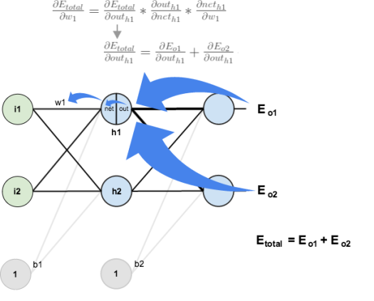
Big picture, here’s what we need to figure out:
$\frac{\partial E_{total}}{\partial w_{1}} = \frac{\partial E_{total}}{\partial out_{h1}} * \frac{\partial out_{h1}}{\partial net_{h1}} * \frac{\partial net_{h1}}{\partial w_{1}}$
Visually:

We’re going to use a similar process as we did for the output layer, but slightly different to account for the fact that the output of each hidden layer neuron contributes to the output (and therefore error) of multiple output neurons. We know that $out_{h1}$ affects both $out_{o1}$ and $out_{o2}$ therefore the $\frac{\partial E_{total}}{\partial out_{h1}}$ needs to take into consideration its effect on the both output neurons:

$\frac{\partial E_{total}}{\partial out_{h1}} = \frac{\partial E_{o1}}{\partial out_{h1}} + \frac{\partial E_{o2}}{\partial out_{h1}}$

Starting with $\frac{\partial E_{o1}}{\partial out_{h1}}$ :
$\frac{\partial E_{o1}}{\partial out_{h1}} = \frac{\partial E_{o1}}{\partial net_{o1}} * \frac{\partial net_{o1}}{\partial out_{h1}}$

We can calculate $\frac{\partial E_{o1}}{\partial net_{o1}}$ using values we calculated earlier:
$\frac{\partial E_{o1}}{\partial net_{o1}} = \frac{\partial E_{o1}}{\partial out_{o1}} * \frac{\partial out_{o1}}{\partial net_{o1}} = 0.74136507 * 0.186815602 = 0.138498562$

And $\frac{\partial net_{o1}}{\partial out_{h1}}$ is equal to $w_5$ :
$net_{o1} = w_5 * out_{h1} + w_6 * out_{h2} + b_2 * 1$
$\frac{\partial net_{o1}}{\partial out_{h1}} = w_5 = 0.40$

Plugging them in:
$\frac{\partial E_{o1}}{\partial out_{h1}} = \frac{\partial E_{o1}}{\partial net_{o1}} * \frac{\partial net_{o1}}{\partial out_{h1}} = 0.138498562 * 0.40 = 0.055399425$

Following the same process for $\frac{\partial E_{o2}}{\partial out_{o1}}$ , we get:
$\frac{\partial E_{o2}}{\partial out_{h1}} = -0.019049119$

Therefore:
$\frac{\partial E_{total}}{\partial out_{h1}} = \frac{\partial E_{o1}}{\partial out_{h1}} + \frac{\partial E_{o2}}{\partial out_{h1}} = 0.055399425 + -0.019049119 = 0.036350306$

Now that we have $\frac{\partial E_{total}}{\partial out_{h1}}$ , we need to figure out $\frac{\partial out_{h1}}{\partial net_{h1}}$ and then $\frac{\partial net_{h1}}{\partial w}$ for each weight:
$out_{h1} = \frac{1}{1+e^{-net_{h1}}}$
$\frac{\partial out_{h1}}{\partial net_{h1}} = out_{h1}(1 - out_{h1}) = 0.59326999(1 - 0.59326999 ) = 0.241300709$

We calculate the partial derivative of the total net input to $h_1$ with respect to $w_1$ the same as we did for the output neuron:
$net_{h1} = w_1 * i_1 + w_2 * i_2 + b_1 * 1$
$\frac{\partial net_{h1}}{\partial w_1} = i_1 = 0.05$

Putting it all together:
$\frac{\partial E_{total}}{\partial w_{1}} = \frac{\partial E_{total}}{\partial out_{h1}} * \frac{\partial out_{h1}}{\partial net_{h1}} * \frac{\partial net_{h1}}{\partial w_{1}}$
$\frac{\partial E_{total}}{\partial w_{1}} = 0.036350306 * 0.241300709 * 0.05 = 0.000438568$

You might also see this written as:
$\frac{\partial E_{total}}{\partial w_{1}} = (\sum\limits_{o}{\frac{\partial E_{total}}{\partial out_{o}} * \frac{\partial out_{o}}{\partial net_{o}} * \frac{\partial net_{o}}{\partial out_{h1}}}) * \frac{\partial out_{h1}}{\partial net_{h1}} * \frac{\partial net_{h1}}{\partial w_{1}}$
$\frac{\partial E_{total}}{\partial w_{1}} = (\sum\limits_{o}{\delta_{o} * w_{ho}}) * out_{h1}(1 - out_{h1}) * i_{1}$
$\frac{\partial E_{total}}{\partial w_{1}} = \delta_{h1}i_{1}$

We can now update $w_1$ :
$w_1^{+} = w_1 - \eta * \frac{\partial E_{total}}{\partial w_{1}} = 0.15 - 0.5 * 0.000438568 = 0.149780716$

Repeating this for $w_2$ , $w_3$ , and $w_4$
$w_2^{+} = 0.19956143$
$w_3^{+} = 0.24975114$
$w_4^{+} = 0.29950229$

Finally, we’ve updated all of our weights! When we fed forward the 0.05 and 0.1 inputs originally, the error on the network was 0.298371109. After this first round of backpropagation, the total error is now down to 0.291027924. It might not seem like much, but after repeating this process 10,000 times, for example, the error plummets to 0.000035085. At this point, when we feed forward 0.05 and 0.1, the two outputs neurons generate 0.015912196 (vs 0.01 target) and 0.984065734 (vs 0.99 target).